This one’s mostly a big pile of stuff about negative probability, which I made a bit of progress thinking about this month. This time I went for the approach of just calculating a bunch of things to see if that would help, and it sort of did – I came across a way of thinking about where the negative probabilities come from that I haven’t seen before. I’ve written up what I found below. Writing up always takes longer than I expect, so I ran out of time to cover much else, though there’s a couple of other short sections at the end.

I’m planning to eventually use this as the basis for a blog post, so if you read it I’d really appreciate some feedback! This is a first draft that I wrote down in the order it came into my head, but it’s not necessarily the best order for understanding, so any comments on organisation would be useful. Also please tell me about typos, mathematical errors, or anything that could be explained better, so that I can do a better job the second time round. Or ask questions. Or anything else you want, really.

If you’re not interested in negative probability, skip right to the bottom and there’s a couple of short sections about The Master and His Emissary and other stuff I’ve been reading/doing.

Negative probability

I spent some time this month looking for examples with simple numbers. I make a lot of arithmetic errors while calculating, and as I was trying the approach of ‘just calculating a bunch of things’ I wanted to make things as easy for myself as possible. Also, I’m going to be giving a short talk on negative probabilities at this workshop in August, and it’s only 20 minutes, so I wanted to find an example that’s as simple as possible so I can reasonably cover it in the time. I was going to use a qubit example, but even there the numbers are slightly messy. 

Then I remembered this blog post by Dan Piponi, which has a clever and unusually straightforward example. The exact situation in this example doesn’t happen in quantum mechanics, but conceptually it’s very similar, and the numbers are nice and simple.

It’s short and very well described in the post, so it might be a good idea to just switch to reading that first. I’m going to explain it again here, but I’ll use a bit more formalism because I want to extend the discussion to some other examples, so my version might feel more clunky and won’t get to the point as fast. Anyway, the setup for his example is the following:

… a machine produces boxes with (ordered) pairs of bits in them, each bit viewable through its own door.

We’ll call them Box A and Box B. So there are four possibilities for the overall state:

• Box A in state 0, Box B in state 0
• Box A in state 0, Box B in state 1
• Box A in state 1, Box B in state 0
• Box A in state 1, Box B in state 1

We can write these out as a 2×2 grid:

Now there are three questions you can ask about the state which each give you one bit of information:

• Question 0: Is Box A in state 0?
• Question 1: Is Box B in state 0?
• Question 2: Are the boxes both in the same state?

If you remember me talking about van Enk’s extension of the Spekkens toy model ages ago, or about the Wigner function for qubit states, these questions might look familiar. In fact, I’m going to write everything out in his terminology – this is probably overkill and I’ll hopefully be able to drop it for the blog post once I’ve written this first draft. But I’ve been finding it helpful even for thinking about simple examples, so I’ll use it below.

In van Enk’s formalisation there are two variables and , which can each take the value 0 or 1. Question 0 asks about the state of the variable . Question 1 asks about the state of the variable . Question 2 asks about the state of the variable , with the extra detail that we’re taking the addition mod 2, so 1+1=0.

Example 1: good old positive probabilities

Before I get to Piponi’s example I’ll go through one that isn’t strange and counterintuitive, and that just uses good old positive probabilities. Imagine that you get the following answers to the questions: yes to question 0, no to question 1, no to question 2. So Box A is in state 0, Box B is in state 1, and the two boxes are in different states. This is all very sensible and consistent.

In van Enk’s terminology we write this as:

The s are three probability distributions, one for each of the three questions, and this says that   with probability 1, with probability 0, and with probability 0.

Now we can also write this a probability distribution over the 2×2 grid drawn above – we’ve learned that it is definitely in the top left one. Following van Enk again, we’ll call this distribution :

 

We can write the s in terms of the s. For example, is the probability of Box A being in state 0, and there are two cells of the grid that contribute to this,   and . Writing this out for all three,

What if we only know the answer to one of the three questions? Well, that constrains you to two of the four cells of the grid. For example, if we only know $Q_0(0) = 1$, then we know it’s definitely on the left side of the grid, but nothing about whether it’s on the top or the bottom:

 

I’ll come back to this idea later, but first let’s go through Piponi’s example. 

Example 2: negative probabilities

In his version, the answers to the questions are: no to question 0, no to question 1, and no to question 2. Or in van Enk’s terminology,  

o Box A is in state 1, Box B is in state 1, and also the boxes are in different states. This is obviously inconsistent! Any two of those answers would give a unique state for both boxes, but all of them together are no good. There’s no sensible underlying distribution that would give rise to all of these answers at once.

But Piponi points out that we can come up with a weird kind of distribution anyway… if we’re prepared to have negative probabilities! We can pick the following:

 

This replicates the s nicely…

$latex Q_0(0) = P(0,0) + P(0,1) = –\frac{1}{2} + \frac{1}{2} = 0$

$latex Q_1(0) = P(0,0) + P(1,0) = –\frac{1}{2} + \frac{1}{2} = 0$

$latex Q_2(0) = P(0,0) + P(1,1) = –\frac{1}{2} + \frac{1}{2} = 0$

… at the cost of apparently not making very much sense. What does a negative probability of mean?

One reassuring result is that you’re never going to actually measure a negative probability. In Piponi’s example you’re only allowed to ask one of the three questions, so you can’t get at any of the s directly. It’s only when you make multiple runs of the experiment with different questions that you find out that the answers are inconsistent. 

Still, the experiment leaves you with a pretty weird set of options: 

If we met such boxes in the real world we’d be forced to conclude that maybe the boxes knew which bit you were going to look at and changed value as a result, or that maybe you didn’t have the free will to choose door that you thought you had, or maybe, even more radically, you’d conclude that the bits generated by the machine were described by negative probabilities.

Mucking around

I’m not going to manage to fully ‘explain’ or ‘interpret’ negative probabilities here. But I do want to go through a way of calculating the s from the s that I haven’t seen explained elsewhere, that makes it less opaque where they come from, and maybe points toward a better understanding of what the negative probabilities could mean.

In Piponi’s post, the s are just pulled out of a hat as numbers that happen to satisfy the questions. Alternatively, you can rearrange the equations for the s in terms of the s, along with the fact that the four s sum to 1, and get some formulae that work but that aren’t necessarily that enlightening on their own.

I spent a while just mucking around with the numbers seeing if I could find something more intuitive, and after a while I came up with something interesting. First off, I’ll rewrite our grid of s as a 2×2 matrix:

This distribution normally gets called   after Wigner… it’s the discrete version of the Wigner function, which I’ve written about before. (But this isn’t all that relevant here, so maybe this is too confusing and in the blog post I should just call it ? That doesn’t come very naturally to me, because I’ve got used to calling some other matrix , but it’s probably better than introducing this random out of nowhere. I really hate notation, it’s the worst.)

(Also I realised after I wrote the whole thing that I cocked up the notation in a more fundamental way. That matrix has   in the bottom left… whereas normally if you’re labelling a matrix the 00 state would be in the top left. This is because I used the same convention as in the picture of the grid I drew, which has the origin in the bottom left. I REALLY hate notation! Anyway it doesn’t affect following the argument at all, it might just be odd if you’re used to things being written out in the normal way.)

Now let’s build up in the following way. Start with complete uncertainty about the state, so that there’s a $latex{1}{4}$ of it being in any state, and then add on corrections after asking the three questions in turn:

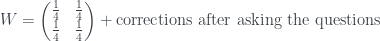
I’ll show how this works for our two examples.

Example 1 again

First ask question 0. We learn that the answer is ‘yes’ (), so this rules out the right hand two cells of the grid and we’re now in the state .

To get there from our initial state of uncertainty, we can add to the entries of the left hand row, and take it away from the right hand row. So this becomes a correction to :

This correction matrix has some negative probabilities in it! They’re fairly innocuous ones, as the result of adding the two matrices has all positive entries. So it’s similar to, say, subtracting the probability of heads from 1 to get the probability of tails, which we’re generally happy with. Still, it’s fun to try and interpret them. We can think of the bottom row of the correction matrix as adding extra probability of those events happening. And we can think of the top row as taking away probability of events happening… or adding probability of them ‘unhappening’.

OK, let’s keep going, and ask question 1. This time the answer is ‘no’ and we need to add on another correction matrix corresponding to that. This correction matrix needs to remove probability from the bottom row and add it to the top row:

Finally, ask question 2, with answer ‘no’:

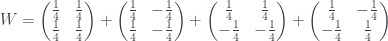
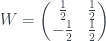
Adding ‘em all up gives

,

I.e. it’s definitely in the top left state, which is what we found before. It’s good to verify that the method works on a conventional example like this, where the final probabilities are positive.

Example 2 again

I’ll follow the same method again for Piponi’s example, starting from complete uncertainty and then adding on a correction for each question (this time the answer is ‘no’ each time). This time I’ll do it all in one go:

which adds up to

Again, we’ve got the same probabilities as Piponi, with the weird negative probability for ‘both in state 0’. We can sort of see why – all three questions rule out this state, so it picks up a term from all of them.

Other stuff I’ve run out of time for

The two examples I did are ones where all three questions have definite yes/no answers, but the method carries over in the obvious way when you have a probability distribution over ‘yes’ and ‘no’. As an example, say you have a 0.8 probability of ‘no’ for question 0. Then you add 0.8 times the correction matrix for ‘no’, with the negative probabilities on the left hand side, and 0.2 times the correction matrix for ‘yes’, with the negative probabilities on the right hand side. Add ‘em all up as before.

I didn’t talk about QM directly, but the method carries over to a qubit state without alteration. There are a couple of extra things you need to think about, though. First, you need to be able to map between this abstract frame of three questions and things you can actually measure. This isn’t so bad – there’s a defined way to relate questions to measurements. (They’re measurements of , where the are the three Pauli matrices, if you care. Though maybe the one also has a factor of i, I haven’t checked.) Second, in QM there’s a constraint on what questions you’re allowed to ask – you’re only allowed to end up with ‘half the information’, according to a slightly weird definition of information I went through back in March last year. This weird definition ends up requiring that the squares of the four s sum to , which you can see is not satisfied for either of the examples we went through. In fact they both sum to 1, which is the definition of having all the information – that makes sense, as there’s a definite answer to all three questions.

Finally, I feel like this whole thing needs more crackpot speculation about events unhappening. Need to think about it more!

 

The Master and His Emissary

I started reading this after getting hyped into it by some of the Less Wrong people. It’s really good so far, and directly relevant to a lot of things I seem to think about endlessly – ‘two types of mathematicians’, decoupling vs contextualising, etc. I don’t have time to say much, but I just want to paste in one quote that is helping me make sense of a few things:

… speaking metaphorically, one might say that language is open to carry us across to the experiential world at the ‘top’ and at the ‘bottom’.

At the ‘top’ end, I am talking about any context – and these are not by any means to be found in poetry alone – in which words are used so as to activate a broad net of connotations, which though present to us, remains implicit, so the meanings are appreciated as a whole, at once, to the whole of our being, conscious and unconscious, rather than being subject to the isolating effects of sequential, narrow-beam attention. As long as they remain implicit, they cannot be hijacked by the conscious mind and turned into just another series of worn paraphrase. If this should happen, the power is lost, much like a joke that has to be explained (humour is a right-hemisphere faculty).

At the ‘bottom’ end, I am talking about the fact that every word, in and of itself, eventually has to lead us out of the web of language, to the lived world, and ultimately to something that can only be pointed to, something that relates to our embodied existence… Everything has to be expressed in terms of something else, and those something elses eventually have to come back to the body. To change the metaphor (and invoke the spirit of Wittgenstein) that is where one’s spade reaches bedrock and is turned. There is nothing more fundamental in relation to which we can understand that.

I’ve been muddling those for a while, and it’s really helpful to get them separated out like this. When I wrote the cognitive decoupling elite post I was mostly thinking about the second one (but not in a way where I’d really consciously separated them). I was thinking of coupling in very much the way that physicists would use the term, like actual forces pulling on you from things in the world and making them show up as directly relevant to you, and I wasn’t especially considering language at all. 

John Nerst’s version of the decoupling idea (the one that took off) was interesting, because it was clearly the same sort of thing, it didn’t feel at all like he’d misinterpreted me, but it felt weirdly different in tone to what I was going for in a way I struggled to articulate. I’d now say it was mostly about the ‘top’ end of language, and the connections between things that are already partially abstracted as verbal statements, whereas I was mainly thinking about the ‘bottom’ end.

(As a comparison, I also got a response from Raymond Finzel linking me to this post of his, and the first part is pretty much exactly what I was going for – the world as ‘both inherently useful and inherently emotional’. This stuff seems to be mostly preverbal, I think.)

Other things this month

• I put up all the old 2018 newsletters on my blog here. Seems like I’m happy making them public after a lag.
• I tried the ‘blogs and Twitter on Thursdays and Fridays only’ rule, and it mostly just annoyed me. Felt very arbitrary and constraining in the same way restricting to specific times of day did, and I mostly stopped doing it. I did stay off Twitter, though.
•  Didn’t read outside my normal internet as much as last month, but I did come across a few interesting things:
  • I read this old GOFAIish paper that seems to be the original source of the decoupling idea, and learned how to pretend a banana is a telephone
  • I read some more Schwitzgebel, who I first came across last month. Nice example: Disorder in the Representational Warehouse.
  • ‘Postmodern products’. There’s been quite a few articles in this line after that Peppa Pig one in 2017, but this one linking bizarre algorithmically generated Amazon storefronts to some evangelical church via many other weird intermediaries is fantastic. 
  • I also found another good postmodern product via tumblr, the ‘Chinooks and Chinstrap Penguins’ colouring book: 

Somebody wrote an algorithm to steal photos from Google Image Search and other zero-cost sources, run them through a series of Photoshop filters, and package them up into “coloring books”. They then dumped an alphabetised list of animal names into it and walked away, and human oversight was either too absent or too indifferent to pick up on the fact that all of the top image search results for “chinook” were for aircraft rather than fish – and the result is a shitty colouring book full of deep fried JPEG artifacts with the utterly inexplicable subject matter pairing of cute penguins and military transport helicopters. Like, this is it. This is the inassailable culmination of everything deep-fried memes aspire to be, and it was devised by a brainless machine. We live in the stupidest cyberpunk future, and it is awesome.

Next month

• I’ll keep going with this negative probability thing, and at least start on drafting a blog post.
• I’m going to a quantum foundations summer school in Zurich!
• No more new internet rules for this month, as I seem to have temporarily run out of steam for that kind of thing.

Cheers,

Lucy