This is Part 2 of a two part explanation — Part 1 is here. It won’t make much sense on its own!
In this post I’m going to get into the details of the analogy I set up last time. So far I’ve described how the PR box is ‘worse than quantum physics’ in a specific sense: it violates the CHSH inequality more strongly than any quantum system, pushing past the Tsirelson bound of to reach the maximum possible value of 4. I also introduced Piponi’s box example, another even simpler ‘worse than quantum physics’ toy system.
This time I’ll explain the connection between Piponi’s box and qubit phase space, and then show that a similar CHSH-inequality-like ‘logical Bell inequality’ holds there too. In this case the quantum system has a Tsirelson-like bound of , interestingly intermediate between the classical limit of 1 and the maximum possible value of 3 obtained by Piponi’s box. Finally I’ll dump a load of remaining questions into a Discussion section in the hope that someone can help me out here.
A logical Bell inequality for the Piponi box
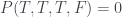
Here’s the table from the last post again:
Measurement
T
F
1
0
1
0
1
0
As with the PR box, we can use the yellow highlighted cells in the table to get a version of Abramsky and Hardy’s logical Bell inequality , this time with cells. These cells correspond to the three incompatible propositions , with combined probability , violating the inequality by the maximum amount.
Converting to expected values gives
.
So that’s the Piponi box ↔ PR box part of the analogy sorted. Next I want to talk about the qubit phase space ↔ Bell state part. But first it will be useful to rewrite the table of Piponi box results in a way that makes the connection to qubit phase space more obvious:
The four boxes represent the four ‘probabilities’ introduced in the previous post, which can be negative. To recover the values in the table, add up rows, columns or diagonals of the diagram. For example, to find , sum up the left hand column:
.
Or to find , sum up the top-left-to-bottom-right diagonal:
.
I made the diagram below to show how this works in general, and now I’m not sure whether that was a good idea. It’s kind of busy and looking at the example above is probably a lot more helpful. On the other hand, I’ve gone through the effort of making it now and someone might find it useful, so here it is:
Qubit phase space
That’s the first part of the analogy done, between the PR box and Piponi’s box model. Now for the second part, between the CHSH system and qubit phase space. I want to show that the same set of measurements that I used for Piponi’s box also crops up in quantum mechanics as measurements on the phase space of a single qubit. This quantum case also violates the classical bound of , but, as with the Tsirelson bound for an entangled qubit system, it doesn’t reach the maximum possible value. Instead, it tops out at .
The measurements can be instantiated for a qubit in the following way. For a qubit , take
,
,
with for the Pauli matrices . The diagonal measurements then turn out to correspond to
As a simple example, in the case of the qubit state these measurements give
,
leading to the following phase space:
A Tsirelson-like bound for qubit phase space
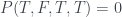
Now, we want to find the qubit state which gives the largest value of . To do this, I wrote out in the general Bloch sphere form and then maximised the value of the highlighted cells in the table:
This is a straightforward calculation but the details are kind of fiddly, so I’ve relegated them to a separate page (like the boring technical appendix at the back of a paper, but blog post style). Anyway the upshot is that this quantity is maximised when , and , leading to the following table:
Measurement
T
F
0
0
0
The corresponding qubit phase space, if you’re interested, is the following:
Notice the negative ‘probability’ in the bottom left, with a value of around -0.183. This is in fact the most negative value possible for qubit phase space.
This time, adding up the numbers in the yellow-highlighted cells of the table gives
,
or, in terms of expectation values,
.
So is our Tsirelson-like bound for this system, in between the classical limit of 1 and the Piponi box value of 3.
Further questions
As with all of my physics blog posts, I end up with more questions than I started with. Here are a few of them:
Is this analogy already described in some paper somewhere? If so, please point me at it!
Numerology. Why and not some other number? As a first step, I can do a bit of numerology and notice that , where is the number of cells in the table, and that this rule also fits the CHSH bound of , where there are cells.
I can also try this formula on the Mermin example from my Bell post. In that case , so the upper bound implied by the rule would be … which turns out to be correct. (I didn’t find the upper bound in the post, but you can get it by putting in all the highlighted cells of the table, similarly to CHSH.)
The Mermin example is close enough to CHSH that it’s not really an independent data point for my rule, but it’s reassuring that it still fits, at least.
What does this mean? Does it generalise? I don’t know. There’s a big literature on different families of Bell results and their upper bounds, and I don’t know my way around it.
Information causality. OK, playing around with numbers is fine, but what does it mean conceptually? Again, I don’t really know my way around the literature. I know there’s a bunch of papers, starting from this one by Pawlowski et al, that introduces a physical principle called ‘information causality’. According to that paper, this states that, for a sender Alice and a receiver Bob,
> the information gain that Bob can reach about the previously unknown to him data set of Alice, by using all his local resources and classical bits communicated by Alice, is at most bits.
This principle somehow leads to the Tsirelson bound… as you can see I have not looked into the details yet. This is probably what I should do next. It’s very much phrased in terms of having two separated systems, so I don’t know whether it can be applied usefully in my case of a single qubit.
If you have any insight into any of these questions, or you notice any errors in the post, please let me know in the comments below, or by email.
I’m still down the rabbithole of thinking way too much about quantum foundations and negative probabilities, and this time I came across an interesting analogy, which I will attempt to explain in this post and the next one. This should follow on nicely from my last post, where I talked about one of the most famous weird features of quantum physics, the violation of the Bell inequalities.
It’s not necessary to read all of that post to understand this one, but you will need to be somewhat familiar with the Bell inequalities (and the CHSH inequality in particular) from somewhere else. For the more technical parts, you’ll also need to know a little bit about Abramsky and Hardy’s logical Bell formulation, which I also covered in the last post. But the core idea probably makes some kind of sense without that background.
So, in that last post I talked about the CHSH inequality and how quantum physics violates the classical upper limit of 2. The example I went through in the post is designed to make the numbers easy, and reaches a value of 2.5, but it’s possible to pick a set of measurements that pushes it further again, to a maximum of (which is about 2.828). This value is known as the Tsirelson bound.
This maximum value is higher than anything allowed by classical physics, but doesn’t reach the absolute maximum that’s mathematically attainable. The CHSH inequality is normally written something like this:
Each of the s has to be between -1 and +1, so if it was possible to always measure +1 for the first three and -1 for the last one you’d get 4.
This kind of hypothetical ‘superquantum correlation’ is interesting because of the potential to illuminate what’s special about the Tsirelson bound – why does quantum mechanics break the classical limit, but not go all the way? So systems that are ‘worse than quantum physics’ and push all the way to 4 are studied as toy models that can hopefully illuminate something about the constraints on quantum mechanics. The standard example is known as the Popescu-Rohrlich (PR) box, introduced in this paper.
This sounds familiar…
I was reading up on the PR box a while back, and it reminded me of something else I looked into. In my blog posts on negativeprobability, I used a simple example due to Dan Piponi. This example has the same general structure as measurements on a qubit, but it’s also ‘worse than quantum mechanics’, in the sense that one of the probabilities is more negative than anything allowed in quantum mechanics. Qubits are somewhere in the middle, in between classical systems and the Piponi box.
I immediately noticed the similarity, but at first I thought it was probably something superficial and didn’t investigate further. But after learning about Abramsky and Hardy’s logical formulation of the Bell inequalities, which I covered in the last post, I realised that there was an exact analogy.
This is really interesting to me, because I had no idea that there was any sort of Tsirelson bound equivalent for a single particle system. I’ve already spent quite a bit of time in the last couple of years thinking about the phase space of a single qubit, because it seems to me that a lot of essential quantum weirdness is hidden in there already, before you even consider entanglement with a second qubit – you’ve already got the negative probabilities, after all. But I wasn’t expecting this other analogy to turn up.
I haven’t come across this result in the published literature. But I also haven’t done anything like a thorough search, and it’s quite difficult to because Piponi’s example is in a blog post, rather than a paper. So maybe it’s new, or maybe it’s too simple to write down and stuck in the ghost library, or maybe it’s all over the place and I just haven’t found it yet. I really don’t know, and it seemed like the easiest thing was to just write it up and then try and find out once I had something concrete to point at. I am convinced it hasn’t been written up at anything like a blog-post-style introductory level, so hopefully this can be useful however it turns out.
Post structure
I decided to split this argument into two shorter parts and post them separately, to make it more readable. This first part is just background on the Tsirelson bound and the PR box – there’s nothing new here, but it was useful for me to collect the background I need in one place. I also give a quick description of Piponi’s box model.
In the second post, I’ll move on to explaining the single qubit analogy. This is the interesting bit!
The Tsirelson bound: Mermin’s machine again
To illustrate how Tsirelson’s bound is attained, I’ll go back to Mermin’s machine from the last post. I’ll use the same basic setup as before, but move the settings on the detectors:
This time the two settings on each detector are at right angles to each other, and the right hand detector settings are rotated 45 degrees from the left hand detector. As before, quantum mechanics says that the probabilities of different combinations of lights flashing will obey
,
,
where is the angle between the detector settings. The numbers are more hassly than Mermin’s example, which was picked for simplicity – here’s the table of probabilities:
Dial setting
(T,T)
(T,F)
(F,T)
(F,F)
Then we follow the logical Bell procedure of the last post, take a set of mutually contradictory propositions (the highlighted cells) and find their combined probability. This gives , or, converting to expectation values ,
.
This is the Tsirelson bound.
The PR box
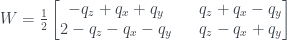
The idea of the PR box is to get the highest violation of the inequality possible, by shoving all of the probability into the highlighted cells, like this:
Dial setting
(T,T)
(T,F)
(F,T)
(F,F)
1/2
0
0
1/2
0
1/2
1/2
0
1/2
0
0
1/2
1/2
0
0
1/2
This time, adding up all the highlighted boxes gives the maximum .
Signalling
This is kind of an aside in the context of this post, but the original motivation for the PR box was to demonstrate that you could push past the quantum limit while still not allowing signalling between the two devices: if you only have access the left hand box, for example, you can’t learn anything about the right hand box’s dial setting. Say you set the left hand box to dial setting . If the right hand box was set to you’d end up measuring T with a probability of
.
If the right hand box was set to instead you’d still get :
.
The same conspiracy holds if you set the left hand box to , so whatever you do you can’t find out anything about the right hand box.
Negative probabilities
Another interesting feature of the PR box, which will be directly relevant here, is the connection to negative probabilities. Say you want to explain the results of the PR box in terms of underlying probabilities for all of the settings at once. This can’t be done in terms of normal probabilities, which is not surprising: this property of having consistent results independent of the measurement settings you choose is exactly what’s broken down for non-classical systems like the CHSH system and the PR box.
However you can reproduce the results if you allow some negative probabilities. In the case of the PR box, you end up with the following:
(I got these from Abramsky and Brandenburger’s An Operational Interpretation of Negative Probabilities and No-Signalling Models.) To get back the probabilities in the table above, sum up all relevant Ps for each dial setting. As an example, take the top left cell of the table above. To get the probability of (T,T) for dial setting (a,b), sum up all cases where a and b are both T:
In this way we recover the values of all the measurements in the table – it’s only the s that are negative, not anything we can actually measure. This feature, along with the way that the number crops up specifically, is what reminded me of Piponi’s blog post.
Piponi’s box model
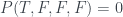
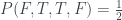
The device in Piponi’s example is a single box containing two bits and , and you can make one of three measurements: the value of , the value of , or the value of . The result is either T or F, with probabilities that obey the following table:
Measurement
T
F
1
0
1
0
1
0
These measurements are inconsistent and can’t be described with any normal probabilities , but, as with the PR box, they can with negative probabilities:
For example, the probability of measuring and getting F is
,
as in the table above.
Notice that crops up again! The similarities to the PR box go deeper, though. The PR box is a kind of extreme version of the CHSH state of two entangled qubits – same basic mathematics but pushing the correlations up higher. Analogously, Piponi’s box is an extreme version of the phase space for a single qubit. In both cases, quantum mechanics is perched intriguingly in the middle between classical mechanics and these extreme systems. I’ll go through the details of the analogy in the next post.
This post is a long, idiosyncratic discussion of the Bell inequalities in quantum physics. There are plenty of good introductions already, so this is a bit of a weird thing to spend my time writing. But I wanted something very specific, and couldn’t find an existing version that had all the right pieces. So of course I had to spend far too much time making one.
My favourite introduction is Mermin’s wonderful Quantum Mysteries for Anyone. This is an absolute classic of clear explanation, and lots of modern pop science discussions derive from it. It’s been optimised for giving a really intense gut punch of NOTHING IN THE WORLD MAKES SENSE ANY MORE, which I’d argue is the main thing you want to get out of learning about the Bell inequalities.
However, at some point if you get serious you’ll want to actually calculate things, which means you’ll need to make the jump from Mermin’s version to the kind of exposition you see in a textbook. The most common modern version of the Bell inequalities you’ll see is the CHSH inequality, which looks like this:
(It doesn’t matter what all of that means, at the moment… I’ll get to that later.) The standard sort of derivations of this tend to involve a lot of fussing with algebraic rearrangements and integrals full of s and so forth. The final result is less of a gut punch and more of a diffuse feeling of unease: “well I guess this number has to be between -2 and 2, but it isn’t”.
This feels like a problem to me. There’s a 1929 New Yorker cartoon which depicts ordinary people in the street walking around dumbstruck by Einstein’s theory of general relativity. This is a comic idea because the theory was famously abstruse (particularly back then when good secondary explanations were thin on the ground). But the Bell inequalities are accessible to anyone with a very basic knowledge of maths, and weirder than anything in relativity. I genuinely think that everyone should be walking down the street clutching their heads in shock at the Bell inequalities, and a good introduction should help deliver you to this state. (If you don’t have rocks in your head, of course. In that case nothing will help you.)
It’s also a bit of an opaque black box. For example, why is there a minus sign in front of one of the s but not the others? I was in a discussion group a few years back with a bunch of postdocs and PhD students, all of us with a pretty strong interest in quantum foundations, and CHSH came up at some point. None of us had much of a gut sense for what that minus sign was doing… it was just something that turned up during some algebra.
I wanted to trace a path from Mermin’s explanation to the textbook one, in the hope of propagating some of that intuitive force forward. I wrote an early draft of the first part of this post for a newsletter in 2018 but couldn’t see how to make the rest of it work, so I dropped it. This time I had a lot more success using some ideas I learned in the meantime. I ended up taking a detour through a third type of explanation, the ‘logical Bell inequalities’ approach of Abramsky and Hardy. This is a general method that can be used on a number of other similar ‘no-go theorems’, not just Bell’s original. It gives a lot more insight into what’s actually going on (including that pesky minus sign). It’s also surprisingly straightforward: the main result is a few steps of propositional logic.
That bit of propositional logic is the most mathematically involved part of this post. The early part just requires some arithmetic and the willingness to follow what Mermin calls ‘a simple counting argument on the level of a newspaper braintwister’. No understanding of the mathematics of quantum theory is needed at all! That’s because I’m only talking about why the results of quantum theory are weird, and not how the calculations that produce those results are done.
If you also want to learn to do the calculations, starting from a basic knowledge of linear algebra and complex numbers, I really like Michael Nielsen and Andy Matuschak’s Quantum Country, which covers the basic principles of quantum mechanics and also the Bell inequalities. You’d need to do the ‘Quantum computing for the very curious’ part, which introduces a lot of background ideas, and then the ‘Quantum mechanics distilled’ part, which has the principles and the Bell stuff.
There’s also nothing about how the weirdness should be interpreted, because that is an enormous 90-year-old can of rotten worms and I would like to finish this post some time in my life 🙂
Mermin’s machine
So, on to Mermin’s explanation. I can’t really improve on it, and it would be a good idea to go and read that now instead, and come back to my version afterwards. I’ve repeated it here anyway though, partly for completeness and partly because I’ve changed some notation and other details to mesh better with the Abramsky and Hardy version I’ll come to later.
(Boring paragraph on exactly what I changed, skip if you don’t care: I’ve switched Mermin’s ‘red’ and ‘green’ to ‘true’ and ‘false’, and the dial settings from 1,2,3 on both sides to on the left side and on the right side. I’ve also made one slightly more substantive change. Mermin explains at the end of his paper that in his setup, ‘One detector flashes red or green according to whether the measured spin is along or opposite to the field; the other uses the opposite color convention’. I didn’t want to introduce the complication of having the two detectors with opposite wiring, and have made them both respond the same way, flashing T for along the field and F for opposite. But I also wanted to keep Mermin’s results. To do that I had to change the dial positions of the right hand dial, so that is opposite , is opposite , and is opposite . )
Anyway, Mermin introduces the following setup:
The machine in the middle is the source. It fires out some kind of particle – photons, electrons, frozen peas, whatever. We don’t really care how it works, we’ll just be looking at why the results are weird.
The two machines on the right and left side are detectors. Each detector has a dial with three settings. On the left they’re labelled , and . On the right, they’re , and .
On the top of each are two lights marked T and F for true and false. (Again, we don’t really care what’s true or false, we’re keeping everything at a kind of abstract, operational level and not going into the practical details. It’s just two possible results of a measurement.)
It’s vital to this experiment that the two detectors cannot communicate at all. If they can, there’s nothing weird about the results. So assume that a lot of work has gone into making absolutely sure that the detectors are definitely not sharing information in any way at all.
Now the experiment just consists of firing out pairs of particles, one to each detector, with the dials set to different values, and recording whether the lights flash red or green. So you get a big list of results of the form
The second important point, other than the detectors not being able to communicate, is that you have a free choice of setting the dials. You can set them both beforehand, or when the particles are both ‘in flight’, or even set the right hand dial after the left hand detector has already received its particle but before the right hand particle gets there. It doesn’t matter.
Now you do like a million billion runs of this experiment, enough to convince you that the results are not some weird statistical fluctuation, and analyse the results. You end up with the following table:
Dial setting
(T,T)
(T,F)
(F,T)
(F,F)
1/2
0
0
1/2
1/8
3/8
3/8
1/8
1/8
3/8
3/8
1/8
1/8
3/8
3/8
1/8
1/2
0
0
1/2
1/8
3/8
3/8
1/8
1/8
3/8
3/8
1/8
1/8
3/8
3/8
1/8
1/2
0
0
1/2
Each dial setting has a row, and the entries in that row give the probabilities for getting the different results. So for instance if you set the dials to and , there’s a 1/8 chance of getting (T,T).
This doesn’t obviously look particularly weird at first sight. It only turns out to be weird when you start analysing the results. Mermin condenses two results from this table which are enough to show the weirdness. The first is:
Result 1: This result relates to the cases where the two dials are set to , , or . In these cases both lights always flash the same colour. So you might get , , etc, but never or .
This is pretty easy to explain. The detectors can’t communicate, so if they do the same thing it must be something to do with the properties of the particles they are receiving. We can explain it straightforwardly by postulating that each particle has an internal state with three properties, one for each dial position. Each of these takes two possible values which we label T or F. We can write these states as e.g.
where the the entries on the top line refer to the left hand particle’s state when the dial is in the , and positions respectively, and the bottom line refers to the right hand particle’s state when the dial is in the , , position.
Result 1 implies that the states of the two particles must always be the same. So the state above is an allowed one, but e.g.
isn’t.
Mermin says:
This hypothesis is the obvious way to account for what happens in [Result 1]. I cannot prove that it is the only way, but I challenge the reader, given the lack of connections between the devices, to suggest any other.
Because the second particle will always have the same state to the first one, I’ll save some typing and just write the first one out as a shorthand. So the first example state will just become TTF.
Now on to the second result. This one covers the remaining options for dial settings, , and the like.
Result 2: For the remaining states, the lights flash the same colour 1/4 of the time, and different colours 3/4 of the time.
This looks quite innocuous on first sight. It’s only when you start to consider how it meshes with Result 1 that things get weird.
(This is the part of the explanation that requires some thinking ‘on the level of a newspaper braintwister’. It’s fairly painless and will be over soon.)
Our explanation for result 1 is that particles in each run of the experiment have an underlying state, and both particles have the same state. Let’s go through the implications of this, starting with the example state TTF.
I’ve enumerated the various options for the dials in the table below. For example, if the left dial is and the right dial is , we know that the left detector will light up T and the right will light up T, so the two lights are the same.
Dial setting
Lights
same
different
same
different
different
different
Overall there’s a 1/3 chance of being the same and a 2/3 chance of being different. You can convince yourself that this is also true for all the states with two Ts and an F or vice versa: TTF TFF, TFT, FTT, FTF, FFT.
That leaves TTT and FFF as the other two options. In those cases the lights will flash the same colour no matter what the dial is set to.
So whatever the underlying state is, the chance of the two lights being different is greater than ⅓. But this is incompatible with Result 2, which says that the probability is ¼.
(The thinky part is now done.)
So Results 1 and 2 together are completely bizarre. No assignment of states will work. But this is exactly what happens in quantum mechanics!
You probably can’t do it with frozen peas, though. The details don’t matter for this post, but here’s a very brief description if you want it: the particles should be two spin-half particles prepared in a specific ‘singlet’ state, the dials should connect to magnets that can be oriented in three states at 120 degree angles from each other, and the lights on the detectors measure spin along and opposite to the field. The magnets should be set up so that the state for setting on the left hand side is oriented at 180 degrees from the state for setting on the right hand side; similarly should be opposite and opposite . I’ve drawn the dials on the machine to match this. Quantum mechanics then says that the probabilities of the different results are
where is the angle between the magnet states on the left and right sides. This reproduces the numbers in the table above.
Once more with less thinking
Mermin’s argument is clear and compelling. The only problem with it is that you have to do some thinking. There are clever details that apply to this particular case, and if you want to do another case you’ll have to do more thinking. Not good. This is where Abramsky and Hardy’s logical Bell approach comes in. It requires more upfront setup (so actually more thinking in the short term – this section title is kind of a lie, sorry) but can then be applied systematically to all kinds of problems.
This first involves reframing the entries in the probability table in terms of propositional logic. For example, we can write the result (T,F) for (a’,b) as . Then the entries of the table correspond to the probabilities we assign to each statement: in this case, .
Now, look at the following highlighted cells in three rows of the grid:
Dial setting
(T,T)
(T,F)
(F,T)
(F,F)
1/2
0
0
1/2
1/8
3/8
3/8
1/8
1/8
3/8
3/8
1/8
1/8
3/8
3/8
1/8
1/2
0
0
1/2
1/8
3/8
3/8
1/8
1/8
3/8
3/8
1/8
1/8
3/8
3/8
1/8
1/2
0
0
1/2
These correspond to the three propositions
,
which can be written more simply as
.
where the stands for logical equivalence. This also means that can be substituted for , and so on, which will be useful in a minute.
Next, look at the highlighted cells in these three rows:
Now it can be shown quite quickly that these six propositions are mutually contradictory. First use the first three propositions to get rid of , and , leaving
You can check that these are contradictory by drawing out the truth table, or maybe just by looking at them, or maybe by considering the following stupid dialogue for a while (this post is long and I have to entertain myself somehow):
Grumpy cook 1: You must have either beans or chips but not both.
Me: OK, I’ll have chips.
Grumpy cook 2: Yeah, and also you must have either beans or peas but not both.
Me: Fine, looks like I’m having chips and peas.
Grumpy cook 3: Yeah, and also you must have either chips or peas but not both.
Me: …
Me: OK let’s back up a bit. I’d better have beans instead of chips.
Grumpy cook 1: You must have either beans or chips but not both.
Me: I know. No chips. Just beans.
Grumpy cook 2: Yeah, and also you must have either beans or peas but not both.
Me: Well I’ve already got to have beans. But I can’t have them with chips or peas. Got anything else?
Grumpy cook 3: NO! And remember, you must have either chips or peas.
Me:hurls tray
So, yep, the six highlighted propositions are inconsistent. But this wouldn’t necessarily matter, as some of the propositions are only probabilistically true. So you could imagine that, if you carefully set some of them to false in the right ways in each run, you could avoid the contradiction. However, we saw with Mermin’s argument above that this doesn’t save the situation – the propositions have ‘too much probability in total’, in some sense, to allow you to do this. Abramsky and Hardy’s logical Bell inequalities will quantify this vague ‘too much probability in total’ idea.
Logical Bell inequalities
This bit involves a few lines of logical reasoning. We’ve got a set of propositions (six of them in this example case, in general), each with probability . Let be the probability of all of them happening together. Call this combined statement
.
Then
where the second equivalence is de Morgan’s law. This is definitely less than the sum of the probabilities of all the s:
.
where is the total number of propositions. Rearranging gives
.
Now suppose the are jointly contradictory, as in the Mermin example above, so that the combined probability . This gives the logical Bell inequality
.
This is the precise version of the ‘too much probability’ idea. In the Mermin case, there are six propositions, three with probability 1 and three with probability ¾, which sum to 5.25. This is greater than , so the inequality is violated.
This inequality can be applied to lots of different setups, not just Mermin’s. Abramsky and Hardy use the CHSH inequality mentioned in the introduction to this post as their first example. This is probably the common example used to introduce Bell’s theorem, though the notation is usually somewhat different. I’ll go though Abramsky and Hardy’s version and then connect it back to the standard textbook notation.
The CHSH inequality
The CHSH experiment only uses two settings on each side, not three. I’ve drawn a ‘CHSH machine’ in the style of Mermin’s machine to illustrate it:
There are two settings and on the left side, 60 degrees apart. And there are two settings and on the right side, also 60 degrees apart, with opposite . This leads to the following table:
Dial setting
(T,T)
(T,F)
(F,T)
(F,F)
1/2
0
0
1/2
3/8
1/8
1/8
3/8
3/8
1/8
1/8
3/8
1/8
3/8
3/8
1/8
Now it’s just a case of following the same reasoning as for the Mermin case. The highlighted rows correspond to the propositions
As with Mermin’s example, these four propositions can be seen to be contradictory. Rather than trying to make up more stupid dialogues, I’ll just follow the method in the paper. First use to replace with in :
Then use to swap out again, this time with :
Finally use to swap out with , leaving
which is clearly contradictory.
(Sidenote: I guess these sort of arguments to show a contradiction do involve some thinking, which is what I was trying to avoid earlier. But in each case you could just draw out a truth table, which is a stupid method that a computer could do. So I think it’s reasonable to say that this is less thinking than Mermin’s method.)
Again, this violates the logical Bell inequality. In total, we have
.
The textbook version of this inequality is a bit different. For a start, it uses an ‘expectation value’ for each proposition rather than a straightforward probability, where truth is associated with +1 and falsity with -1. So each proposition has an expectation value with
Then summing over the s gives
and then, using the previous form of the logical Bell inequality,
.
A similar argument for shows that , so that this is a bound above and below:
.
In this case and so the inequality becomes . However adding up the s associated to the propositions gives 2.5, so the inequality is violated.
There’s still a little further to go to get the textbook version, but we’re getting close. The textbook version writes the CHSH inequality as
.
where the expectation value is written in the form
.
The are ‘hidden variables’ – properties of the particles that dispose them to act in various ways. For example, in the Mermin case, we imagined them to have hidden states, like
that controlled their response to each dial, and showed that any choice of these hidden states would lead to a contradiction.
For a given , and are the values measured by the left and right hand machines respectively. In our case these values are always either +1 (if the machine flashes T) or -1 (if the machine flashes F). The CHSH argument can also be adapted to a more realistic case where some experimental runs have no detection at all, and the outcome can also be 0, but this simple version won’t do that.
For the dial settings and , all we care about with these hidden variables is whether they make the machines respond true or false. So in our case is just a set of four variables, , and the integral can just become a sum:
.
.
Now that first proposition is just from earlier, which had probability . And the second one covers all the remaining possibilities, so it has probability . So
.
The argument goes through exactly the same way for and . The last case, , is slightly different. We get
following the same logic as before. But this time matches the second proposition , not the first, so that
.
This is where the minus sign in the CHSH inequality comes in! We have
.
So we end up with the standard inequality, but with a bit more insight into where the pieces come from. Also, importantly, it’s easy to extend to other situations. For example, you could follow the same method with the six Mermin propositions from earlier to make a kind of ‘Mermin-CHSH inequality’:
.
Or you could have three particles, or a different set of measurements, or you could investigate what happens with other tables of correlations that don’t appear in quantum physics… this is a very versatile setup. The original paper has many more examples.
Final thoughts
There are still some loose ends that it would be good to tie up. I’d like to understand exactly how the inequality-shuffling in a ‘textbook-style’ proof of the CHSH inequality connects to Abramsky and Hardy’s version. Presumably some of it is replicating the same argument, but in a more opaque form. But also some of it must need to deal with the fact that it’s a more general setting, and includes things like measurements returning 0 as well as +1 or -1. It would be nice to figure out which bits are which. I think Bell’s original paper didn’t have the zero thing either, so that could be one place to look.
On the other hand… that all sounds a bit like work, and I can’t be bothered for now. I’d rather apply some of this to something interesting. My next post is probably going to make some connections between the logical Bell inequalities and my previous twoposts on negative probability.
If you know the answers to my questions above and can save me some work, please let me know in the comments! Also, I’d really like to know if I’ve got something wrong. There are a lot of equations in this post and I’m sure to have cocked up at least one of them. More worryingly, I might have messed up some more conceptual points. If I’ve done that I’m even more keen to know!
OK, so this is where I go back through everything from the last post, but this time show how all the fiddling around with boxes relates back to quantum physics, and also go into some technical details like explaining what I meant by ‘half the information’ in the discussion at the end. This is unavoidably going to need more maths than the last post, and enough quantum physics knowledge to be OK with qubits and density matrices. I’ll start by translating everything into a standard physics problem.
Qubit phase space
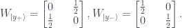
So, first off, instead of the ‘strange machine’ of the last post we will have a qubit state – as a first example I’ll take the state. The three questions then become measurements on it. Specifically, these measurements are expectation values of the operators , where the are the three Pauli matrices.
For we get the following:
This can be represented on the same sort of 2×2 grid I used in the previous post:
The state has a definite value of 0 for the measurement, so the probabilities in the cells where must sum to 1. For the state there is an equal chance of either or . The third measurement, , can be shown to be associated with the diagonals of the grid, in the same way as in Piponi’s example in the previous post, and again there is an equal chance of either value. Imposing all these conditions gives the probability assignment above.
The 2×2 grid is called the phase space of the qubit, and the function that assigns probabilities to each cell is called the Wigner function. To save on drawing diagrams, I’ll represent this as a square-bracketed matrix from now on:
For much more detail on how this all works, the best option is probably to read Wootters, who developed a lot of the ideas in the first place. There’s his original paper, which has all the technical details, and a nice follow-up paper on Picturing Qubits in Phase Space which gives a bit more intuition for what’s going on.
In the previous post I gave the following formula for the Wigner function:
which simplifies to
This is a somewhat different form to the standard formula for the Wigner function, but I’ve checked that they’re equivalent. I’ve put the details on a separate notes page here, in a sort of blog post version of the really boring technical appendix you get at the back of papers.
Magic states
As with the example in the last blog post, it’s possible to get qubit states where some of the values of the Wigner function are negative. The numbers don’t work out so nicely this time, but as one example we can take the qubit state . (This is the +1 eigenvector of the density matrix .)
The Wigner function for is
with one negative entry. I learned while writing this that the states with negative values are called magic states by quantum computing people! These are the states that provide the ‘magic’ for quantum computing, in terms of giving a speed-up over classical computing. I’d like be able to say more about this link, but I’ll never finish the post if I have to get my head around all of that too, so instead I’ll link to this post by Earl Campbell that goes into more detail and points to some references. A quick note on the geometry, though:
The six eigenvectors of the Pauli matrices form the corners of an octahedron on the Bloch sphere, as in my dubious sketch above. We’ve already seen that the state has no magic – all the values are nonnegative. This also holds for the other five, which have the following Wigner functions:
The other states on the surface of the octahedron or inside it also have no magic. The magic states are the ones outside the octahedron, and the further they are from the octahedron the more magic they are. So the most magic states are on the surface of the sphere opposite the middle of the triangular faces.
Half the information
Why can’t we have a probability of as before? Well, I briefly mentioned the reason in the previous blog post, but I can go into more detail now. There are constraints on the values of that forbids values that are this negative. First off, the values of have to sum to 1 – this makes sense, as they are supposed to be something like probabilities.
The second constraint is more interesting. Taking the state as an example again, this state has a definite answer to one of the questions and no information at all about the other two. There’s redundancy in the questions, so exact answers to two of them would be enough to pin down the state precisely. So we have half of the possible information.
This turns out to be the most information you can get from any qubit state, in some sense. I say ‘in some sense’ because it’s a pretty odd definition of information.
I learned about this from a fascinating paper by van Enk, A toy model for quantum mechanics, which was actually my starting point for thinking about this whole topic. He starts with the Spekkens toy model, a very influential idea that reproduces a number of the features of quantum mechanics using a very simple model. Again, this is too big a topic to get into all the details, but the most basic system in this model maps to the six ‘non-magic’ qubit states listed above, in the corners of the octahedron. These all share the half-the-knowledge property of the state, where we know the answer to one question exactly and have no idea about the others.
Now van Enk’s aim is to extend this idea of ‘half the knowledge’ to more general probability distributions over the four boxes. But this requires having some kind of measure of what half the knowledge means. He stipulates that this measure should have for the six half-the-knowledge states we already have, which seems reasonable. Also, it should have for states where we know all the information (impossible in quantum physics), and for the state of total ignorance about all questions. Or to put it a bit differently,
,
where is an entropy measure – it decreases from 2 to 1 to 0 as we learn more information about the system. There’s a parametrised family of entropies known as the Rényi entropies, which reproduce this behaviour for the cases above, and differ for other distributions over the boxes. (I have some rough notes about these here, which may or may not be helpful.) By far the most well-known one is the Shannon entropy, used widely in information theory, but it turns out that this one doesn’t reproduce the states found in quantum physics. Instead, van Enk picks , the collision entropy. This has quite a simple form:
,
where the are the four components of – we’re just summing the squares of them. So then our information measure is just , and the second constraint on is this can have value at most :
.
Why this particular entropy measure? That’s something I don’t really understand. Van Enk describes it as ‘the measure of information advocated by Brukner and Zeilinger’, and links to their paper, but so far I haven’t managed to follow the argument there, either. If anyone reads this and has any insight, I’d like to know!
Questions
In some ways, I know a lot more about negative probabilities than I did when I started getting interested in this. But conceptually I’m almost as confused as I was at the start! I think the main improvement is that I have some more focussed questions to be confused about:
Is the way of decomposing the Wigner function that I described in these posts any use for making sense of the negative probabilities? I found it quite helpful for Piponi’s example, in giving some more insight into how the negative value connects to that particular answer being ‘especially inconsistent’. Is it also useful for thinking about qubits?
Any link to the idea of negative probabilities representing events ‘unhappening’? As I said at the beginning of the first post, I love this idea but have never seen it fully developed anywhere in a satisfying way.
What’s going on with this collision entropy measure anyway?
I’m not a quantum foundations researcher – I’m just an interested outsider trying to understand how all these ideas fit together. So I’m likely to be missing a lot of context that people in the field would have. If you read this and have pointers to things that I’m missing, please let me know in the comments!
I’ve been thinking about the idea of negative probabilities a lot recently, and whether it’s possible to make any sense of them. (For some very muddled and meandering background on how I got interested in this, you could wade through my ramblings here, here, here and here, but thankfully none of that is required to understand this post.)
To save impatient readers the hassle of reading this whole thing: I’m not going to come up with any brilliant way of interpreting negative probabilities in this blog post! But recently I did notice a few things that are interesting and that I haven’t seen collected together anywhere else, so I thought it would be worth writing them up.
Now, why would you even bother trying to make sense of negative probabilities? I’m not going to go into this in any depth – John Baez has an great introductory post on negative probability that motivates the idea, and links to a good chunk of the (not very large) literature. This is well worth reading if you want to know more. But there are a couple of main routes that lead people to get interested in this thing.
The first route is pretty much pure curiosity: what happens if we try extending the normal idea of probabilities to negative numbers? This is often introduced in analogy with the way we often use negative numbers in applications to simplify calculations. For example, there’s a fascinating discussion of negative probability by Feynman which starts with the following simple situation:
A man starting a day with five apples who gives away ten and is given eight during the day has three left. I can calculate this in two steps: 5 – 10 = -5 and -5 + 8 = 3.
The final answer is satisfactorily positive and correct although in the intermediate steps of calculation negative numbers appear. In the real situation there must be special limitations of the time in which the various apples are received and given since he never really has a negative number, yet the use of negative numbers as an abstract calculation permits us freedom to do our mathematical calculations in any order, simplifying the analysis enormously, and permitting us to disregard inessential details.
So, although we never actually have a negative number of apples, allowing them to appear in intermediate calculations makes the maths simpler.
The second route is that negative probabilities actually crop up in exactly this way in quantum physics! This isn’t particularly obvious in the standard formulation learned in most undergrad courses, but the theory can also be written in a different way that closely resembles classical statistical mechanics. However, unlike the classical case, the resulting ‘distribution’ is not a normal probability distribution, but a quasiprobability distribution that can also take negative values.
As with Feynman’s apples, these negative values don’t map to anything we observe directly: all measurements we could make give results that occur with zero or positive probabilities, as you would expect. The negative probabilities instead come in as intermediate steps in the calculation.
This should become clearer when I work through a toy example. The particular example I’ll use (which I got from an excellent blog post by Dan Piponi) doesn’t come up in quantum physics, but it’s very close: its main advantage is that the numbers are a bit simpler, so it’s easier to concentrate on the ideas. I’ll do this in two pieces: one that requires no particular physics or maths background and just walks through the example using basic arithmetic, and one that makes connections back to the quantum mechanics literature and might drop in a Pauli matrix or two. This is the no-maths one.
Neither of these routes really get to the point of fully making sense of negative probabilities. In the apple example, we have a tool for making calculations easier, but we also have an interpretation of ‘a negative apple’, in terms of taking away one of the apples you have already. For negative probabilities, we mostly just have the calculational tool. It’s tempting to try and follow the apple analogy and interpret negative probabilities as being to do with something like ‘events unhappening’ – many people have suggested this (see e.g. Michael Nielsen here), and I certainly share the intuition that something like this ought to be possible, but I’ve never seen anything fully worked out along those lines that I’ve found really satisfying.
In the absence of a compelling intuitive explanation, I find it helpful to work through examples and get an idea of how they work. Even if we don’t end up with a good explanation for what negative probabilities are, we can see what they do, and start to build up a better understanding of them that way.
A strange machine
OK, so let’s go through Piponi’s example (here’s the link again). He describes it very clearly and concisely in the post, so it might be a good idea to just switch to reading that first, but for completeness I’ll also reproduce it here.
Piponi asks us to consider a case where:
a machine produces boxes with (ordered) pairs of bits in them, each bit viewable through its own door.
So you could have 0 in both boxes, 0 in the first and 1 in the second, and so on. Now suppose we ask the following three questions about the boxes:
Is the first box in state 0?
Is the second box in state 0?
Are the boxes both in the same state?
I’ll work through two possible sets of answers to these questions: one consistent and unobjectionable set, and one inconsistent and stupid one.
Example 1: consistent answers
Let’s say that we find that the answer to the first question is ‘yes’ , the answer to the second is ‘no’, and the answer to the third is ‘no’. This makes sense, and we can interpret this easily in terms of an underlying state of the two boxes. The first box is in state 0, the second box is in state 1, and so of course the two are in different states and the answer to the third question is also satisfied.
We can represent this situation with the grid below:
The system is in state ‘first box 0, second box 1’, with probability 1, and the other states have probability 0. This is all very obvious – I’m just labouring the point so I can compare it to the case of inconsistent answers, where things get weird.
Example 2: inconsistent answers
Now suppose we find a inconsistent set of answers when we measure the box: ‘no’ to all three questions. This doesn’t make much intuitive sense: both boxes are in state 1, but also they are in different states. Still, Piponi demonstrates that you can still assign something like ‘probabilities’ to the squares on the grid, as long as you’re OK with one of them being negative:
Let’s go through how this matches up with the answers to the questions. For the first question, we have
so the answer is ‘no’ as required. Similarly, for the other two questions we have
and
so we get ‘no’ to all three, at the expense of having introduced this weird negative probability in one cell of the grid.
It’s not obvious at all what the negative probability means, though! Piponi doesn’t explain how he came up with this solution, but I’m guessing it’s one of either ‘solve the equations and get the answer’ or ‘notice that these numbers happen to work’.
I wanted to think a bit more about interpretation, and although I haven’t fully succeeded, I did notice a more enlightening calculation method, which maybe points in a useful direction. I’ll describe it below.
A calculation method
Some motivating intuition: all four possible assignments of bits to boxes are inconsistent with the answers in Example 2, but ‘both bits are zero’ is particularly inconsistent. It’s inconsistent with the answers to all three questions, whereas the other assignments are inconsistent with only one question each (for example, ‘both bits are 1’ matches the answer to the first two questions, but is inconsistent with the two states being different).
So you can maybe think in terms of consecutively answering the three questions and penalising assignments that are inconsistent. ‘Both bits are zero’ is an especially bad answer, so it gets clobbered three times instead of just once, pushing the probability negative.
The method I’ll describe is a more formal version of this. I’ll go through it first for Example 1, with consistent answers, to show it works there.
Back to Example 1
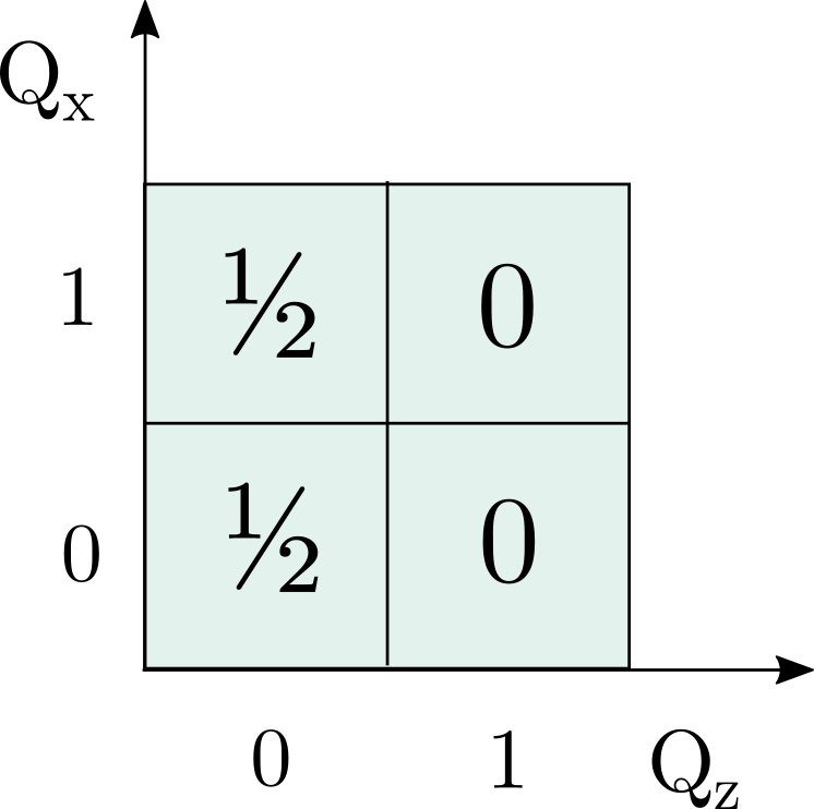
Imagine that we start in a state of complete ignorance. We have no idea what the underlying state is, so we just assign probability ¼ to each cell of the grid, like this:
(I’ll stop drawing the axes every time from this point on.) We then ask the three questions in succession and make corrections. For the first question, ‘is the first box in state 0’, we have the answer ‘yes’, so after we learn this we know that the left two cells of the grid now have probability ½ each, and the right two have probability 0. We can think of this as adding a correction term to our previous state of ignorance:
Notice that the correction term has some negative probabilities in it! But these seem relatively benign from an interpretational point of view – they are just removing probability from some cells so that it can be reassigned to others, and the final answer is still positive. It’s kind of similar to saying , where we subtract some probability to get to the answer.
Next, we add on two more correction terms, one for each of the remaining two questions. The correction term for the second question needs to remove probability from the bottom row and add it to the top row, and the one for the third question corrects the diagonals:
Adding ‘em all up gives
So the system is definitely in the top left state, which is what we found before. It’s good to verify that the method works on a conventional example like this, where the final probabilities are positive.
Example 2 again
I’ll follow the same method again for Piponi’s example, starting from complete uncertainty and then adding on a correction for each question (this time the answer is ‘no’ each time). This time I’ll do it all in one go:
which adds up to
So we’ve got the same probabilities as Piponi, with the weird negative -½ probability for ‘both in state 0’. This time we get a little bit more insight into where it comes from: it’s picking up a negative correction term from all three questions.
Discussion
This ‘strange machine’ looks pretty bizarre. But it’s extremely similar to a situation that actually comes up in quantum physics. I’ll go into the details in the follow-up post (‘now with added equations!’), but this example almost replicates the quasiprobability distribution for a qubit, one of the simplest systems in quantum physics. The main difference is that Piponi’s machine is slightly ‘worse’ than quantum physics, in that the -½ value is more negative than anything you get there.
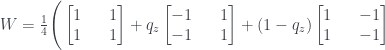
The two examples I did were ones where all three questions have definite yes/no answers, but my method of starting from a state of ignorance and adding on corrections carries over in the obvious way when you have a probability distribution over ‘yes’ and ‘no’. As an example, say you have a 0.8 probability of ‘no’ for the first question. Then you add 0.8 times the correction matrix for ‘no’, with the negative probabilities on the left hand side, and 0.2 times the correction matrix for ‘no’, with the negative probabilities on the right hand side. That’s all there is to it. Just to spell it out I’ll add the general formula: if the three questions have answer ‘no’ with probabilities , , respectively, then we assign probabilities to the cells as follows:
(If you’re wondering where the comes from, it’s just the usual letter used to label this thing – it stands for ‘Wigner’, and is a discrete version of his Wigner function.)
It turns out that all examples in quantum physics are of the type where you don’t have certain knowledge of the answers to all three questions. It’s possible to know the answer to one of them for certain, but then you have to be completely ignorant about the other two, and assign probability ½ to both answers. More usually, you will have partial information about all three questions, with a constraint that the total information you get about the system is at most half the total possible information, in a specific technical sense. To go into this in detail will require some more maths, which I’ll get to in the next post.
My second favourite type of question in physics, after ‘what’s the simplest non-trivial example of this thing?’, is probably ‘how can I write these two things in the same formalism, so that the differences stand out more clearly?’
This may look like an odd choice, given that all I ever do here is grumble about how crap I am at picking up new formal techniques. But actually that’s part of why I like it!
Writing two theories in the same language is like putting two similar transparencies on top of each other, and holding them up to the light. Suddenly the genuine conceptual differences pop out visibly, freed from the distraction of all the tedious extraneous machinery that surrounds them.
Or at least that’s always the hope – it’s actually pretty hard work to do this.
There are two maps between classical and quantum physics that I’m interested in learning, and should probably have included in my crackpot grand plan. (I guess they can be shoved into the quantum foundations grab bag.)
One is the phase space reformulation of quantum mechanics. This is sort of a standard technique, but I still managed to avoid hearing about it until quite recently. Some subfields apparently use it a lot, but you’re unlikely to see it in any standard quantum course. It also has a weird lack of decent introductory texts. I met someone at the workshop I went to who uses it in their research and asked what I should read, and he just looked pained and said ‘My thesis, maybe? When I write it?’ So learning it may not be especially fun.
It looks really interesting though! You can dump all the operators and use something that looks very like a normal probability distribution, so the parallels with classical statistical mechanics are much more explicit. There are obviously differences – this distribution can be negative, for a start. (It’s known as a quasidistribution.) Ideally, I’d like to be able to hold them both up to the light and see exactly where all the differences are.
It’s less well known that you can also do classical mechanics on Hilbert space! It’s called Koopman – von Neumann theory. If you ever thought ‘what classical mechanics is really missing is a load of complex wavefunctions on configuration space’, then this is the formalism for you.
In this case, I ought to be luckier with the notes, because Frank Wilczek wrote some a couple of years ago.
I’m not so clear on exactly what this thing is and what I’d get out of learning it, but the novelty value of a Born rule in classical mechanics is high enough that I can’t resist giving it a go. And I’d have a new pair of formalisms to hold up to the light.


 s has to be between -1 and +1, so if it was possible to always measure +1 for the first three and -1 for the last one you’d get 4.
 ,
, ,
, is the angle between the detector settings. The numbers are more hassly than Mermin’s example, which was picked for simplicity – here’s the table of probabilities:


 , or, converting to expectation values
  ,
, .
.


 .
. .
. instead you’d still get
  :
: .
. , so whatever you do you can’t find out anything about the right hand box.
 for all of the settings at once. This can’t be done in terms of normal probabilities, which is not surprising: this property of having consistent results independent of the measurement settings you choose is exactly what’s broken down for non-classical systems like the CHSH system and the PR box.


 s that are negative, not anything we can actually measure. This feature, along with the way that the number
  crops up specifically, is what reminded me of Piponi’s blog post.


 ,
, crops up again! The similarities to the PR box go deeper, though. The PR box is a kind of extreme version of the CHSH state of two entangled qubits – same basic mathematics but pushing the correlations up higher. Analogously, Piponi’s box is an extreme version of the phase space for a single qubit. In both cases, quantum mechanics is perched intriguingly in the middle between classical mechanics and these extreme systems. I’ll go through the details of the analogy in the next post.
 s and so forth. The final result is less of a gut punch and more of a diffuse feeling of unease: “well I guess this number has to be between -2 and 2, but it isn’t”.
 on the left side and
  on the right side. I’ve also made one slightly more substantive change. Mermin explains at the end of his paper that in his setup, ‘One detector flashes red or green according to whether the measured spin is along or opposite to the field; the other uses the opposite color convention’. I didn’t want to introduce the complication of having the two detectors with opposite wiring, and have made them both respond the same way, flashing T for along the field and F for opposite. But I also wanted to keep Mermin’s results. To do that I had to change the dial positions of the right hand dial, so that
  is opposite
  , and
, and  is opposite
  . )
. )
 and
and  . On the right, they’re
  and
and  .
.


 , or
, or  . In these cases both lights always flash the same colour. So you might get
  ,
,  ,
,  etc, but never
  or
or  .
.

 and the like.

 . Then the entries of the table correspond to the probabilities we assign to each statement: in this case,
  .
.

 ,
,

 .
. stands for

 ,
,

 .
. stands for


 (six of them in this example case,
  in general), each with probability
  . Let
. Let  .
.
 s:
s:

 .
. .
. . This gives the logical Bell inequality
 .
. , so the inequality is violated.


 to replace
  :
:
 to swap out
 to swap out
 .
. with
with

 .
. shows that
  , so that this is a bound above and below:
 .
. and so the inequality becomes
  . However adding up the
  .
.
 and
and  are the values measured by the left and right hand machines respectively. In our case these values are always either +1 (if the machine flashes T) or -1 (if the machine flashes F). The CHSH argument can also be adapted to a more realistic case where some experimental runs have no detection at all, and the outcome can also be 0, but this simple version won’t do that.
 , and the integral can just become a sum:
 .
. .
. is just
  . And the second one covers all the remaining possibilities, so it has probability
  . So
. So .
. and
and  . The last case,
  , is slightly different. We get
 , not the first, so that
 .
. .
. .
. of the operators
  , where the

 measurement, so the probabilities in the cells where
  must sum to 1. For the
  state there is an equal chance of either
  or
or  . The third measurement,
  , can be shown to be associated with the diagonals of the grid, in the same way as in Piponi’s example in the previous post, and again there is an equal chance of either value. Imposing all these conditions gives the probability assignment above.
  . To save on drawing diagrams, I’ll represent this as a square-bracketed matrix from now on:
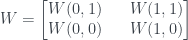

 . (This is the +1 eigenvector of the density matrix
  .)
.)  is
is 

 state has no magic – all the values are nonnegative. This also holds for the other five, which have the following Wigner functions:
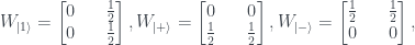
 of what half the knowledge means. He stipulates that this measure should have
  for the six half-the-knowledge states we already have, which seems reasonable. Also, it should have
  for states where we know all the information (impossible in quantum physics), and
  for the state of total ignorance about all questions. Or to put it a bit differently,
 ,
, is an entropy measure – it decreases from 2 to 1 to 0 as we learn more information about the system. There’s a parametrised family
  of entropies known as the
  , used widely in information theory, but it turns out that this one doesn’t reproduce the states found in quantum physics. Instead, van Enk picks
  , the collision entropy. This has quite a simple form:
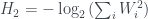 ,
, are the four components of
  , and the second constraint on
  .
.


 , where we subtract some probability to get to the answer.


 ,
,  ,
,  respectively, then we assign probabilities to the cells as follows:
